This article is just brief summary of Generative Adversarial Nets (Goodfellow et al., NIPS 2014) and posting for me to study what is the GAN(Generative Adversarial Networks).
First of all, This GAN(Genrative Adversarial Nets) is a framework which explains adversarial training for recover traing data distribution, In this paepr, The generator G implicitly defines a probability distribution \( p_{g} \) as the distribution of the samples \( G(z) \) when \( z \sim p_{z} \).
Let’s see the objective funtion of the GAN.
\( \min_{G} \max_{D} V(G,D) = \mathbb{E} {x \sim p_{data}(x)} [logD(x)] + \mathbb{E} {z \sim p_{z}(z)}[log(1-D(G(z))] \)
As you can see above, G and D play two-player minmax game with value function V(G,D).
More specifically,
- Generator network : try to fool the discriminative by generating real-looking data like image and text and so on.
- Discriminative network : try to distinguish between real and fake data like image and text and so on.
traing G and D to their goal, G generates fake data which is similar more and more to real data, whereas D discriminate between fake and real data.
So The G and D complementarily help improve the performance of each other.
-
Discrimanator wants to maximize objective such that D(x) is close to 1(real) and D(G(z)) is close to 0(fake)
-
Generator wants to minimize objective such that D(G(z)) is close to 1 for discriminator to be fooled into thinking generated G(z) is real.
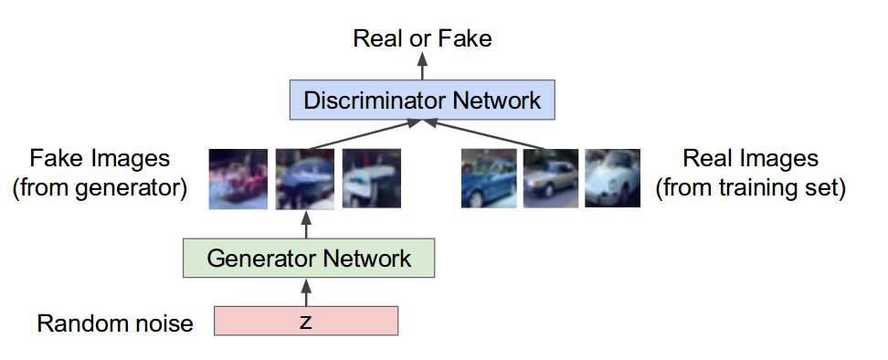
In this paper, both of G and D is multiplayer perceptrons and the output of function V(G,D) is a scalar where measures whether the sample is from traning data or from sample generator create.
There is the following problem where you use the funtion V(G,D) as it is.
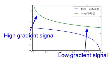
As you can see above, the original equation may not provide the sufficient gradient for G to learn well as it is in the figure above. So in the paper, they suggest other eqaution for G like this:
Early in learing, \( log(1-D_{\theta_{d}}(G_{\theta_{g}}(z)) \) saturates, that’s why the original equation is hard for G to learn well.
In the paper, they used a trick. it maximzes log(D(G(z))) rather than minimize log(1-D(G(z))) like the upper curve in the figure above.
Let’s see some figure in GAN paper about explaining how for GAN to be trained.
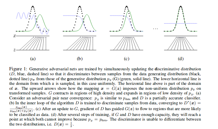
As you can see above, each line means like this :
-
D, blue, dashed line : updating discirminative distribution
-
back, dotted line \( p_{x} \) : data generating distribution
-
green, solid line \( p_{g}(G) \) : genrative distribution
-
The horizontal line above is part of the domain of x
-
The horizontal line below is the domain from which z is sampled.
-
The upward arrows show how the mapping x = G(z) imposes the non-uniform distribution \( p_{g} \) on the transformed samples.
(a), (b), (c) and (d) in turn update the adversarial traing. (a) currently discriminative doesn’t be trained. (b) the discriminator is trained so the blue dotted line is chaneg.
(c) After uan update of G (d) After several steps of tranining, it is ideal step, where \( p_{data} = p_{g} \). The discriminator is not able to distinguish between the two distribution. i.e. D(x) = 1/2.
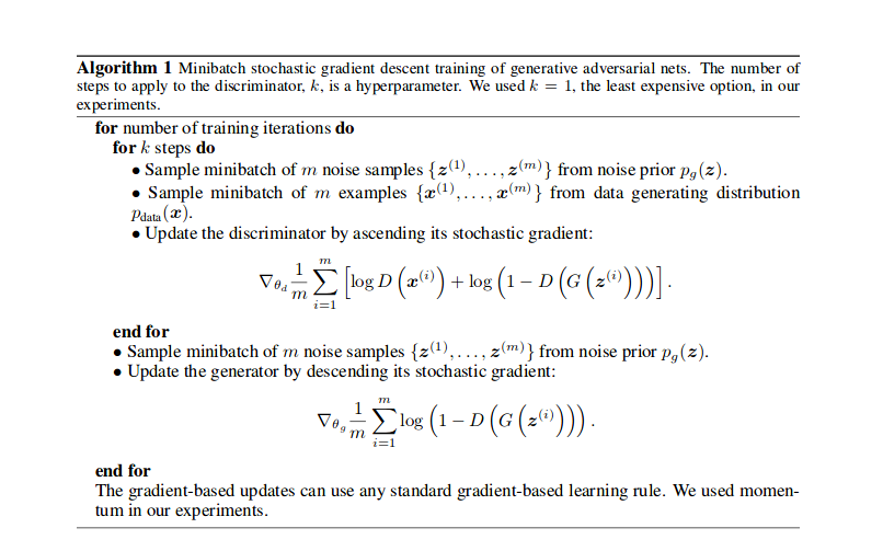
The algorithm of adversarial trainig is the following :
The following is just mathematical analysis of GAN peper equation. if you want to know more, read But if not, skipping is good.
From now on, go through theoretical results they argue about GAN
The theoretical results is based on a non parametric setting.
Proposition 1. For G fixed, the optimal discriminator D is \( D_{G}^{*}(x) = p_{data}(x) / (p_{data}(x) + p_{g}(x)) \)
proof. The trainig criterion for the discriminator D, given any generator G, is to maximize the quantity V(G, D)
\( V(G, D) = \int_{x} p_{data}(x)log(D(x))dx + \int_{z} p_{z}(z)log(1-D(g(z)))dz \) \( V(G, D) = \int_{x} p_{data}(x)log(D(x))dx + p_{g}(x)log(1 - D(x))dx \)
In the eqaution, Expected value of latent value z changes into data space x by using generator that estimate the data distribution with latent variable z.
V(G, D) could be simply expressed like this:
For any (a,b) \( \in \mathbb{R^{2}} \) , the function y -> a*log(y) + b*log(1-y) achieves maximum value in [0,1] at a/(a+b).
if you get derivative of the function y -> a*log(y) + b*log(1-y) with respect to y for \( argmax_{y} f(y) \), suppose the base of logarithms above is e.
y’ = a/y - b/(1-y) and when y’ = 0, the value of y is a point for maxmimum value of y.
0 = a/y - b/(1-y)
0 = a(1-y) - by
(a+b)*y = a
y = a/(a+b)
the funtion y -> a*log(y) + b*log(1-y) reaches maximum in [0,1] at a/(a+b).
\( \min_{G} \max_{D} V(G,D) = \mathbb{E} {x \sim p_{data}(x)} [logD(x)] + \mathbb{E} {z \sim p_{z}(z)} [log(1-D(G(z))] \) is reformulated as :
\( C(G) = \max_{D} V(G,D) \) \( = \mathbb{E} {x \sim p_{data}} [log(D_{G}^{*}(x))] + \mathbb{E} {z \sim p_{z}} [log(1-D_{G}^{*}(G(z)))] \) \( = \mathbb{E} {x \sim p_{data}} [log(D_{G}^{*}(x))] + \mathbb{E} {x \sim p_{g}} [log(1-D_{G}^{*}(x))] \) \( = \mathbb{E} {x \sim p_{data}} [log(p_{data}(x) / (p_{data}(x) + p_{g}(x)))] + \mathbb{E} {x \sim p_{g}} [log(p_{g}(x) / (p_{data}(x) + p_{g}(x)))]) \)
Therorem 1. The global minimum of the virtual training criterion C(G) is achivied if and only if \( p_{g} = p_{data} \). At the point, C(G) reaches the value -log4.
proof. for \( p_{g} = p_{data}, p_{data}(x) / (p_{data}(x) + p_{g}(x)) = p_{g}(x) / (p_{data}(x) + p_{g}(x)) = 1/2 \), C(G) is equal to :
\( \mathbb{E} {x \sim p_{data}} [-log2] + \mathbb{E} {x \sim p_{g}} [-log2] = -log4 \)
and then if you subtract -log4 from \( C(G) = V(D_{G}^{*}, G) \), we obatain :
\( C(G) = -log4 + log4 + \mathbb{E} {x \sim p_{data}} [log(p_{data}(x) / (p_{data}(x) + p_{g}(x)))] + \mathbb{E} {x \sim p_{g}} [log(p_{g}(x) / (p_{data}(x) + p_{g}(x)))] \) \( =-log4 + \mathbb{E} {x \sim p_{data}} [log(p_{data}(x) / (p_{data}(x) + p_{g}(x)))] + log2 + \mathbb{E} {x \sim p_{g}}[log(p_{g}(x) / (p_{data}(x) + p_{g}(x)))] + log2 \) \( = -log4 + KL(p_{data} || (p_{data}+p_{g})/2) + KL(p_{g} || (p_{data}+p_{g})/2)) \)
and then, \( JSD(P || Q) = 1/2*D_{KL} (P||M) + 1/2*D_{KL} (Q||M) \) where M = (P+Q)/2
so, \( C(G) = -log4 + 2*JSD(p_{data} || p_{g}) \).
Since Jensen-Shanon divergence between two distribution \( JSD(p_{data} || p_{g}) \) is alway non-negative and zero only when they are eqaul.
They showed that C*=-log4 is global minimum of C(G) and the only solution is \( p_{g} = p_{data}. \)
Reference
- Paper
- How to use html for alert
- For your information
- Image Completion with DeepLearning in Tensorflow
- A Beginner’s Guide to Generative Adversarial Networks(GANs)
- Quora of Yann LeCun
- Quora
- GAN Lab
- CS231N slide lecture13 2018
- GAN github1-hwalsuklee/tensorflow-generative-model-collections
- GAN github2-JJashim/GANs-Tensorflow
- GAN github3-wiseodd/generative-models
- GAN github4-revsic/tf-vanilla-gan
- Ian Goodfellow et al.’s Deep Learning Book
- Image Kernel Explained Visually
- Expected value on wikipedia
- Marginal Probability on wikipedia
- Kullback-Leibler divergence on wikipedia
- Korean Ver.