This article is just brief summary of the paper, Extensions of Recurrent Neural Network Language model (Mikolov et al., ICASSP 2011).
This is for me to studying artificial neural network with NLP field.
This paper is extension edition of Their original paper, Recurrent neural Network based language model.
In this paper, they argued their extension led to more than the 15 times speed up with BPTT(backpropagation through time), factorization of output layer, and compression layer.
They said their model can be smaller, faster and mor accurate than the basic one, their original RNN-LM because of the threee factors above.
They also said recurrent neural network can perform clustering of similar histories. i.e. This allows for instance efficient representation of patterns with variable length.
Their simple recurrent neural network is like :
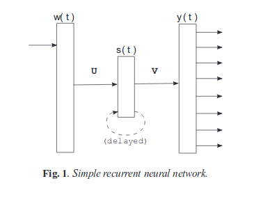
As you can check their original model, recurrent neural network, they here also used sigmoid as activation function in hidden layer and softmax function in output layer as probability distribution function.
They said the BPTT(Backporopagation through time) is extension of the backpropagation algorithm for recurrent networks and with truncated BPTT, the error is propagated through recurrent connections back in time for a pecific number of time steps.
So they were saying the network learned to remember information for several time steps in the hidden layer when it is learned by the BPTT.
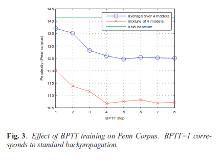
The following figure is the result of BPTT depeding on the number of BPTT steps.
They were also saying the compuational bottlneck is because of the size of vocabularies.
Let’s see the time complexity they said in their paper.
The time complexity of on training step is propotional to
-
\( O = (1+H)*H*t + H*V \) and in this equation, usually \( H << V \), so the computaional bottleneck exists between hiiden and output layer.
- H : the size of the hidden layer
- V : the size of the vocabulary
- t : the amount of steps they backpropagate the error back in time.
As you can see the above equation. because normally computational bottleneck happened between hidden and output layer.
So they introduced factorization of the output layer and compression layer between hidden and output layer.
Factorization of output layer based on the assumption that all words belong to classes.
They mapped all word to exactly one class. Thus they could estimate the probability distribution over the classes using RNN and then calculate the probability of a particular words form the desired class like this:
-
\( P(w_{i} | history) = P(C_{i} | S_{t})P(W_{i} | C_{i}, S_{t}) \)
- \( S_{t} \) : history in context of neural networks that is hidden layer.
The compression layer not only reduces computational complexity, but also reduces the total parameters, which results in the more compact models.
And if the compression layer is between input and hidden layer. it is refered to as a projection layer.
The paper: Extensions of recurrent neural network language model (Mikolov et al., ICASSP 2011)
Reference
- Paper
- Paper for Reference
- How to use html for alert
- For your information