The table of contens in this article.
- Scipy
- Image operations
- MATLAB files
- Distance between points
- Matplotlib
- Plotting
- SubPlots
- Images
Let’s explore more in detail.
Scipy
Numpy provides a high-performance multidimensional array and basic tools to compute with and manipulate these arrrays. Scipy builds on this, and provides a large number of functions that operate on numpy arrays and are useful for different types of scientific and engineering applications.
The best way to get familiar with Scipy is to browse the documentation. We will highlight some parts of Scipy that you might find useful for this class.
Image operations
Scipy provides some basis functions to work with images. For example, it has functions to read images from disk into numpy arrays, to write numpy arrays to disk as images, and to resize images. Here is a simple example that show cases these functions :
>>> import numpy as np
## call of scipy module
>>> from scipy.misc import imread, imsave, imresize
## Read an JPEG image into a numpy array
>>> img = imread('your path of image\cat.jpg')
## img is numpy array, you can verify dtype, ndim, rank, shape and so on
>>> print (type(img))
<class 'numpy.ndarray'>
>>> print (img.dtype, img.shape)
uint8 (400, 248, 3)
>>> img
array([[[132, 128, 117],
        [155, 151, 139],
        [181, 175, 161],
        ...,
        [ 78,  68,  43],
        [ 76,  65,  43],
        [ 64,  53,  31]],

       [[134, 130, 118],
        [152, 148, 136],
        [177, 171, 157],
        ...,
        [ 75,  65,  40],
        [ 72,  61,  39],
        [ 62,  51,  29]],

       [[138, 134, 122],
        [151, 145, 131],
        [174, 168, 152],
        ...,
        [ 71,  61,  36],
        [ 68,  58,  33],
        [ 59,  51,  28]],

       ...,
       [[115, 145,  75],
        [107, 137,  67],
        [106, 135,  69],
        ...,
        [113, 101,  79],
        [106,  94,  72],
        [103,  91,  67]],

       [[107, 134,  65],
        [112, 139,  72],
        [109, 138,  72],
        ...,
        [112,  97,  78],
        [109,  94,  73],
        [101,  89,  67]],

       [[124, 151,  84],
        [116, 143,  76],
        [111, 140,  74],
        ...,
        [ 91,  76,  57],
        [ 89,  74,  55],
        [ 86,  71,  50]]], dtype=uint8)
>>>
###
>>> img_tinted = img * [1, 0.95, 0.9]
>>> imsave('your path to store image\cat_tinted.jpg', img_tinted)
>>> img_tinted = imresize(img_tinted, (300,300))
>>> imsave('your path to store image\cat_tinted_resized.jpg', img_tinted)
img = imread(‘your path of image\cat.jpg’)
print (img.dtype, img.shape)
You can read the image in the above code.

img_tinted = img * [1, 0.95, 0.9]
This only changes RGB of Image.

img_tinted = imresize(img_tinted, (300,300))
This resized image to 300 X 300.

Let’s compare the original image with this resized.
| The original Image | The tinted and resized Image |
|---|---|
|
|
MATLAB files
The function scipy.io.ioloadmat and Scipy.io.savemat allow you to read and write MATLAB files. If you want to know more in detail.
you can read more about the information in the documentation.
Distance between points
Scipy defines some useful functions for computing distances between sets of points.
The function scipy.spatial.distance.pdit computes the distance between all pairs of points in a given set :
\[x = \begin{bmatrix} 0 & 1 \cr 1 & 0 \cr 2 & 0 \cr \end{bmatrix}\]First of all, Create the following array where each row is a point in 2-dimension space :
x = np.array([[0,1],[1,0],[2,0]])
To compute the Euclidean distance between all rows of x.
Use d = squareform(pdist(x, ‘euclidean’))
On the result of squareform function, d[i,j] is the Euclidean distance between x[i,:], and [j, :].
Let’s explain about squareform function slowly.
\[In\ x = \begin{bmatrix} 0 & 1 \cr 1 & 0 \cr 2 & 0 \cr \end{bmatrix},\ suppose\ that\ \begin{bmatrix} 0 \cr 1 \cr \end{bmatrix} = \vec a,\ \begin{bmatrix} 1 \cr 0 \cr \end{bmatrix} = \vec b,\ \begin{bmatrix} 2 \cr 0 \cr \end{bmatrix} = \vec c\] \[\vec a,\ \vec b\ and\ \ \vec c\ are\ in\ Cartesian\ Coordinate\ of\ \rm I\! R^2\]In the above vectors, you can get each distance of them with pdist function.
>>> dis = pdist(x, 'euclidean')
>>> dis
array([ 1.41421356,  2.23606798,  1.        ])
You got one array that is distance of some pairs of points, The pair is element in upper triangular portion of squareform function.
Now, let’s use a function, squareform(pdist(x, ‘euclidean’))
Squareform function makes matrix square as follows.
\[squareform(pdist(x, 'euclidean')) = \begin{bmatrix} 0. & 1.41421356 & 2.23606798 \cr 1.41421356 & 0. & 1. \cr 2.23606798 & 1. & 0. \cr \end{bmatrix}\]In the above matrix, each terms indicate the distance between two points, you can know the location of two points from term index.
if d = squareform(pdist(x, ‘euclidean’)) d[i, j] is the the Euclidean distance between x[i, :] and x[j, :]
d[0, 0] is distance between x[0, :] and x[0, :]
d[0, 1] is distance between x[0, :] and x[1, :]
d[0, 2] is distance between x[0, :] and x[2, :]
…
d[2, 1] is distance between x[2, :] and x[2, :]
d[2, 2] is distance between x[2, :] and x[2, :]
\[In\ x = \begin{bmatrix} 0 & 1 \cr 1 & 0 \cr 2 & 0 \cr \end{bmatrix},\ \begin{bmatrix} 0 \cr 1 \cr \end{bmatrix} = \vec a,\ \begin{bmatrix} 1 \cr 0 \cr \end{bmatrix} = \vec b,\ \begin{bmatrix} 2 \cr 0 \cr \end{bmatrix} = \vec c\]You can come up with which points used from indices
\[d = \begin{bmatrix} 0. & 1.41421356 & 2.23606798 \cr 1.41421356 & 0. & 1. \cr 2.23606798 & 1. & 0. \cr \end{bmatrix}\]d = squareform(pdist(x, ‘euclidean’))
\[0.(d[0, 0])\ is\ distance\ between\ \vec a = \begin{bmatrix} 0 \cr 1 \cr \end{bmatrix}\ and\ \ \vec a = \begin{bmatrix} 0 \cr 1 \cr \end{bmatrix}\] \[1.41421356(d[1, 0])\ is\ distance\ between\ \vec b = \begin{bmatrix} 1 \cr 0 \cr \end{bmatrix}\ and\ \ \vec a = \begin{bmatrix} 0 \cr 1 \cr \end{bmatrix}\] \[2.23606798(d[2, 0])\ is\ distance\ between\ \vec c = \begin{bmatrix} 2 \cr 0 \cr \end{bmatrix}\ and\ \ \vec a = \begin{bmatrix} 0 \cr 1 \cr \end{bmatrix}\]d[i, j] is the Euclidean distance between x[i, :] and x[j, :]
\[pdist(x, 'euclidean') = \begin{bmatrix} 1.41421356 & 2.23606798 & 1. \cr \end{bmatrix}\ \ and\] \[squareform(pdist(x, 'euclidean')) = \begin{bmatrix} 0. & 1.41421356 & 2.23606798 \cr 1.41421356 & 0. & 1. \cr 2.23606798 & 1. & 0. \cr \end{bmatrix}\]Finally, Let’s compare pdist(pdist(x, ‘euclidean’)) with squareform(pdist(x, ‘euclidean’)) once again
If you compare both of them, squareform function makes the result 3 X 3 square, and This matrix will show you distance between a point and self-point.
For example, If you have points, a, b and c. suquareform function also calculates distance between a and a.
But only if you use pdist function. it indicates the distance in order of upper triagular portion of squareform function.
For example, what I meant is as follows :
\[pdist(x, 'euclidean') = \begin{bmatrix} 1.41421356 & 2.23606798 & 1. \cr \end{bmatrix}\ means\] \[1.41421356 = dist(x[0],\ x[1]),\ 2.23606798 = dist(x[0], x[2]),\ 1. = dist(x[1], x[2])\]i.e. You can view it as the elements in the upper triangular portion of the square distance matrix.
Let’s think of what I mean :
\[pdist(x, 'euclidean') = \begin{bmatrix} 1.41421356 & 2.23606798 & 1. \cr \end{bmatrix}\ and\] \[squareform(pdist(x, 'euclidean')) = \begin{bmatrix} 0. & 1.41421356 & 2.23606798 \cr 1.41421356 & 0. & 1. \cr 2.23606798 & 1. & 0. \cr \end{bmatrix}\]Let’s think of it with python code :
>>> dis = pdist(x, 'euclidean')
>>> dis
array([ 1.41421356,  2.23606798,  1.        ])
>>> d = squareform(pdist(x, 'euclidean'))
>>> d
array([[ 0.        ,  1.41421356,  2.23606798],
       [ 1.41421356,  0.        ,  1.        ],
       [ 2.23606798,  1.        ,  0.        ]])

>>> y = np.array([[0,10],[10,10],[20,20],[10,0]])
>>> squareform(pdist(y))
array([[  0.        ,  10.        ,  22.36067977,  14.14213562],
       [ 10.        ,   0.        ,  14.14213562,  10.        ],
       [ 22.36067977,  14.14213562,   0.        ,  22.36067977],
       [ 14.14213562,  10.        ,  22.36067977,   0.        ]])
>>> pdist(y)
array([ 10.        ,  22.36067977,  14.14213562,  14.14213562,
        10.        ,  22.36067977])
If you want to know more in detail, read this Stackoverflow..
Let’s calculate the distance between two points in python code.
>>> import numpy as np
>>> from scipy.spatial.distance import pdist, squareform
>>> x = np.array([[0,1],[1,0],[2,0]])
>>> x
array([[0, 1],
       [1, 0],
       [2, 0]])
>>> print (x)
[[0 1]
 [1 0]
 [2 0]]
>>> d = squareform(pdist(x, 'euclidean'))
>>> d
array([[ 0.        ,  1.41421356,  2.23606798],
       [ 1.41421356,  0.        ,  1.        ],
       [ 2.23606798,  1.        ,  0.        ]])
>>> print (d)
[[ 0.          1.41421356  2.23606798]
 [ 1.41421356  0.          1.        ]
 [ 2.23606798  1.          0.        ]]
>>> d.shape
(3, 3)
>>> d.ndim
2

>>> dis = pdist(x, 'euclidean')
>>> dis
array([ 1.41421356,  2.23606798,  1.        ])
>>> print (dis)
[ 1.41421356  2.23606798  1.        ]
>>> dis.shape
(3,)
>>> dis.ndim
1
You can read all the details about this function in the documentation
A similar function (scipy.spatial.distance.cdist) computes the distance between all paris across sets of points; you can read about it in the documentation
Matplotlib
Matplotlib is a plotting library. In this section, I will give you a brief introduction to the matplotlib.pyplot module, whiich provides a plotting system similar to that of MATLAB.
Plotting
The most important function in matplotlib is plot, which allows you to plot 2D data. Here is a simple example :
>>> import numpy as np
>>> import matplotlib.pyplot as plt
## Compute the x and y coordinates for points on a sine curve
>>> x = np.arange(0, 3 * np.pi, 0.1)
>>> x
array([ 0. ,  0.1,  0.2,  0.3,  0.4,  0.5,  0.6,  0.7,  0.8,  0.9,  1. ,
        1.1,  1.2,  1.3,  1.4,  1.5,  1.6,  1.7,  1.8,  1.9,  2. ,  2.1,
        2.2,  2.3,  2.4,  2.5,  2.6,  2.7,  2.8,  2.9,  3. ,  3.1,  3.2,
        3.3,  3.4,  3.5,  3.6,  3.7,  3.8,  3.9,  4. ,  4.1,  4.2,  4.3,
        4.4,  4.5,  4.6,  4.7,  4.8,  4.9,  5. ,  5.1,  5.2,  5.3,  5.4,
        5.5,  5.6,  5.7,  5.8,  5.9,  6. ,  6.1,  6.2,  6.3,  6.4,  6.5,
        6.6,  6.7,  6.8,  6.9,  7. ,  7.1,  7.2,  7.3,  7.4,  7.5,  7.6,
        7.7,  7.8,  7.9,  8. ,  8.1,  8.2,  8.3,  8.4,  8.5,  8.6,  8.7,
        8.8,  8.9,  9. ,  9.1,  9.2,  9.3,  9.4])
>>> x.shape
(95,)
>>> x.ndim
1
>>> y = np.sin(x)
>>> y
array([ 0.        ,  0.09983342,  0.19866933,  0.29552021,  0.38941834,
        0.47942554,  0.56464247,  0.64421769,  0.71735609,  0.78332691,
        0.84147098,  0.89120736,  0.93203909,  0.96355819,  0.98544973,
        0.99749499,  0.9995736 ,  0.99166481,  0.97384763,  0.94630009,
        0.90929743,  0.86320937,  0.8084964 ,  0.74570521,  0.67546318,
        0.59847214,  0.51550137,  0.42737988,  0.33498815,  0.23924933,
        0.14112001,  0.04158066, -0.05837414, -0.15774569, -0.2555411 ,
       -0.35078323, -0.44252044, -0.52983614, -0.61185789, -0.68776616,
       -0.7568025 , -0.81827711, -0.87157577, -0.91616594, -0.95160207,
       -0.97753012, -0.993691  , -0.99992326, -0.99616461, -0.98245261,
       -0.95892427, -0.92581468, -0.88345466, -0.83226744, -0.77276449,
       -0.70554033, -0.63126664, -0.55068554, -0.46460218, -0.37387666,
       -0.2794155 , -0.1821625 , -0.0830894 ,  0.0168139 ,  0.1165492 ,
        0.21511999,  0.31154136,  0.40484992,  0.49411335,  0.57843976,
        0.6569866 ,  0.72896904,  0.79366786,  0.85043662,  0.8987081 ,
        0.93799998,  0.96791967,  0.98816823,  0.99854335,  0.99894134,
        0.98935825,  0.96988981,  0.94073056,  0.90217183,  0.85459891,
        0.79848711,  0.7343971 ,  0.66296923,  0.58491719,  0.50102086,
        0.41211849,  0.31909836,  0.22288991,  0.12445442,  0.02477543])
>>> y.shape
(95,)
>>> y.ndim
1
### Plot the points using matplotlib
>>> plt.plot(x, y)
[<matplotlib.lines.Line2D object at 0x0523A0D0>]
>>> plt.show()  ## you must call plt.show() to make graphics appear.
After Running this code, the following plot is produced :
.png)
the graph of y = sin(x)
With just a little of extra work, we can easily plot multiple lines at once, and add a title, legend, and axis labels :
>>> import numpy as np
>>> import matplotlib.pyplot as plt
>>>
>>> x = np.arange(0, 3 * np.pi, 0.1)
>>> x
array([ 0. ,  0.1,  0.2,  0.3,  0.4,  0.5,  0.6,  0.7,  0.8,  0.9,  1. ,
        1.1,  1.2,  1.3,  1.4,  1.5,  1.6,  1.7,  1.8,  1.9,  2. ,  2.1,
        2.2,  2.3,  2.4,  2.5,  2.6,  2.7,  2.8,  2.9,  3. ,  3.1,  3.2,
        3.3,  3.4,  3.5,  3.6,  3.7,  3.8,  3.9,  4. ,  4.1,  4.2,  4.3,
        4.4,  4.5,  4.6,  4.7,  4.8,  4.9,  5. ,  5.1,  5.2,  5.3,  5.4,
        5.5,  5.6,  5.7,  5.8,  5.9,  6. ,  6.1,  6.2,  6.3,  6.4,  6.5,
        6.6,  6.7,  6.8,  6.9,  7. ,  7.1,  7.2,  7.3,  7.4,  7.5,  7.6,
        7.7,  7.8,  7.9,  8. ,  8.1,  8.2,  8.3,  8.4,  8.5,  8.6,  8.7,
        8.8,  8.9,  9. ,  9.1,  9.2,  9.3,  9.4])
>>> x.shape
(95,)
>>> x.ndim
1
>>> y_sin = np.sin(y)
>>> y_sin
array([ 0.        ,  0.09983342,  0.19866933,  0.29552021,  0.38941834,
        0.47942554,  0.56464247,  0.64421769,  0.71735609,  0.78332691,
        0.84147098,  0.89120736,  0.93203909,  0.96355819,  0.98544973,
        0.99749499,  0.9995736 ,  0.99166481,  0.97384763,  0.94630009,
        0.90929743,  0.86320937,  0.8084964 ,  0.74570521,  0.67546318,
        0.59847214,  0.51550137,  0.42737988,  0.33498815,  0.23924933,
        0.14112001,  0.04158066, -0.05837414, -0.15774569, -0.2555411 ,
       -0.35078323, -0.44252044, -0.52983614, -0.61185789, -0.68776616,
       -0.7568025 , -0.81827711, -0.87157577, -0.91616594, -0.95160207,
       -0.97753012, -0.993691  , -0.99992326, -0.99616461, -0.98245261,
       -0.95892427, -0.92581468, -0.88345466, -0.83226744, -0.77276449,
       -0.70554033, -0.63126664, -0.55068554, -0.46460218, -0.37387666,
       -0.2794155 , -0.1821625 , -0.0830894 ,  0.0168139 ,  0.1165492 ,
        0.21511999,  0.31154136,  0.40484992,  0.49411335,  0.57843976,
        0.6569866 ,  0.72896904,  0.79366786,  0.85043662,  0.8987081 ,
        0.93799998,  0.96791967,  0.98816823,  0.99854335,  0.99894134,
        0.98935825,  0.96988981,  0.94073056,  0.90217183,  0.85459891,
        0.79848711,  0.7343971 ,  0.66296923,  0.58491719,  0.50102086,
        0.41211849,  0.31909836,  0.22288991,  0.12445442,  0.02477543])
>>> y_sin.shape
(95,)
>>> y_sin.ndim
1
>>> y_cos = np.cos(x)
>>> y_cos
array([ 1.        ,  0.99500417,  0.98006658,  0.95533649,  0.92106099,
        0.87758256,  0.82533561,  0.76484219,  0.69670671,  0.62160997,
        0.54030231,  0.45359612,  0.36235775,  0.26749883,  0.16996714,
        0.0707372 , -0.02919952, -0.12884449, -0.22720209, -0.32328957,
       -0.41614684, -0.5048461 , -0.58850112, -0.66627602, -0.73739372,
       -0.80114362, -0.85688875, -0.90407214, -0.94222234, -0.97095817,
       -0.9899925 , -0.99913515, -0.99829478, -0.98747977, -0.96679819,
       -0.93645669, -0.89675842, -0.84810003, -0.79096771, -0.7259323 ,
       -0.65364362, -0.57482395, -0.49026082, -0.40079917, -0.30733287,
       -0.2107958 , -0.11215253, -0.01238866,  0.08749898,  0.18651237,
        0.28366219,  0.37797774,  0.46851667,  0.55437434,  0.63469288,
        0.70866977,  0.77556588,  0.83471278,  0.88551952,  0.92747843,
        0.96017029,  0.98326844,  0.9965421 ,  0.99985864,  0.99318492,
        0.97658763,  0.95023259,  0.91438315,  0.86939749,  0.8157251 ,
        0.75390225,  0.68454667,  0.60835131,  0.52607752,  0.43854733,
        0.34663532,  0.25125984,  0.15337386,  0.05395542, -0.04600213,
       -0.14550003, -0.24354415, -0.33915486, -0.43137684, -0.51928865,
       -0.6020119 , -0.67872005, -0.74864665, -0.81109301, -0.86543521,
       -0.91113026, -0.9477216 , -0.97484362, -0.99222533, -0.99969304])
>>> y_cos.shape
(95,)
>>> y_cos.ndim
1
>>>
## Plot the points using matplotlib
>>> plt.plot(x, y_sin)
[<matplotlib.lines.Line2D object at 0x0538F070>]
>>> plt.plot(x, y_cos)
[<matplotlib.lines.Line2D object at 0x0538F150>]
>>> plt.xlabel('x axis label')
<matplotlib.text.Text object at 0x07001990>
>>> plt.ylabel('y axis label')
<matplotlib.text.Text object at 0x06CB17D0>
>>> plt.title('Sine and Cosine')
<matplotlib.text.Text object at 0x0536CC30>
>>> plt.legend(['Sine', 'Cosine'])
<matplotlib.legend.Legend object at 0x0538FD10>
>>> plt.show()
let’s see the result of plt.show() :
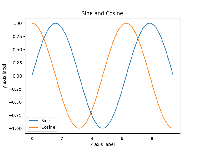
the graph of y_sin and y_cos
you can read much more about the plot function in the documentation
subplot
you can plot different things in the same figure using the subplot function, Here is an example :
>>> import numpy as np
>>> import matplotlib.pyplot as plt
>>>
>>>
>>> x = np.arange(0, 3 * np.pi, 0.1)
>>> y_sin = np.sin(x)
>>> y_cos = np.cos(x)
>>>
## Set up a subplot grid that has height 2 and width 1
## Set first such subplot as active
>>> plt.subplot(2, 1, 1)
<matplotlib.axes._subplots.AxesSubplot object at 0x0539F2F0>
## Make the first plot
>>> plt.plot(x, y_sin)
[<matplotlib.lines.Line2D object at 0x05006C30>]
>>> plt.title('Sine')
<matplotlib.text.Text object at 0x04FEA830>
>>>
## Set the second subplot as active, and Make the second plot
>>> plt.subplot(2,1,2)
<matplotlib.axes._subplots.AxesSubplot object at 0x05006D30>
>>> plt.plot(x, y_cos)
[<matplotlib.lines.Line2D object at 0x0503E790>]
>>> plt.title('Cosine')
<matplotlib.text.Text object at 0x05036790>
>>> plt.xlabel('x')
<matplotlib.text.Text object at 0x05016030>
>>> plt.ylabel('y')
<matplotlib.text.Text object at 0x0501CA30>
>>> plt.legend(['Cosine'])
<matplotlib.legend.Legend object at 0x0503E890>
## Show the figure
>>> plt.show()
>>>
As you can read the above code, after making subplot, each of area is divided.
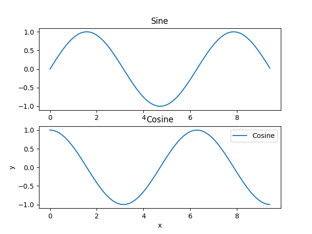
the above is subplot(2,1,1) and the below is subplot(2,1,2)
You can read much mor about the subplot function in the documentation
Images
You can use the imshow function to show image here is an example :
>>> import numpy as np
>>> from scipy.misc import imread, imresize
>>> import matplotlib.pyplot as plt
>>> img = imread('your path including image\cat.jpg')
>>> img_tinted = img * [1, 0.95, 0.9]
## Show the original image
>>> plt.subplot(1,2,1)
<matplotlib.axes._subplots.AxesSubplot object at 0x071A5310>
>>> plt.imshow(img)
<matplotlib.image.AxesImage object at 0x071F1050>
## Show the tinted Image
>>> plt.subplot(1,2,2)
<matplotlib.axes._subplots.AxesSubplot object at 0x071E9FD0>

## If you use plt.imshow(img_tinted), it might give you strange results.
## Then, you explicilty cast the image to unint8 before displaying it.
>>> plt.imshow(np.uint8(img_tinted))                  ## plt.imshow(img_tinted)
<matplotlib.image.AxesImage object at 0x05031770>
>>> plt.show()
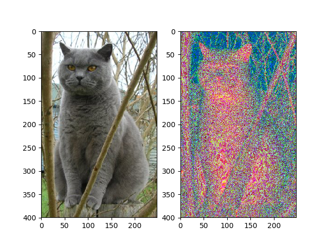
The only case where you use plt.imshow(img_tinted) instead of plt.imshow(np.uint8(img.tinted)
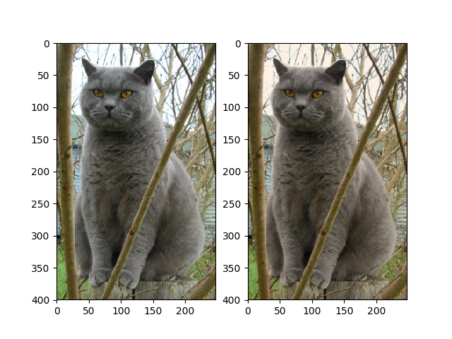
The case where you use correctly plt.imshow(np.unint8(img_tinted)
For a while, you have learned about matplotlib and scipy. But this is so easy.
If you want to know more detail, you need to read reference of scipy or matplotlib api
Reference
For designs of this page
If you want to know more in detail.